- 1 Arithmetic Primitives
- 1.1 Modular Arithmetic Primer
- 1.2 Addition and Subtraction
- 1.3 Multiplication
- 1.4 Division
- 1.5 Exponentiation
- 1.6 Square Root
- 2 Elliptic Curve Cryptography
- 3 Point Operations
- 3.1 Point Addition
- 3.2 Point Doubling
- 3.3 Scalar Point Multiplication
- 3.4 Checking if a point is on curve
- 4 Doing useful ECC operations
- 4.1 Curve cryptosystem parameters
- 4.2 Generating a keypair
- 4.3 Encrypting using ECIES
- 4.4 Signing using ECDSA
- 4.5 Messing with ECDSA signatures
- 5 Advanced Topics
- 6 Examples
- 6.1 Testing your integer arithmetic using Genius
- 6.2 Using Sage to play with elliptic curves
- 6.3 Extracting curve parameters from openssl
- 6.4 Playing with openssl ECDSA signatures
- 6.5 Visualizing a small curve
- 7 FAQ
- 7.1 Cool! Now that I know how to use ECC, should I write my own crypto library?
- 7.2 Can I at least define my own curve then?
- 7.3 But I don't trust NIST/SECG. What alternatives do I have?
- 7.4 Your implementation isn't side channel resistant, hurr durr!
- 8 Downloads
- 9 Literature
1 Arithmetic Primitives
1.1 Modular Arithmetic Primer
One way to do arithmetic calculations is to perform them inside a finite field over a prime number, or Fp. This means that every operation within the basic arithmetic works modulo a chosen prime number. The reason for choosing a prime is that this way, the field has important properties (such as algebraic closure and the invertability of each item within the field). So the basic mathematics is the very same which RSA also uses. It is important to keep one thing in mind when talking about integers, however: Do not just consider integers that fit within your machine word's length, i.e. 64 or 32 bits. When thinking of integer operations that do cryptographic operations, always think of big integers, i.e. 200 or more bits. These have not only to be multiplied, but in some cases also exponentiated. This means some operations are a bit tricky to implement. How this can be done efficiently is described in the next few sections.1.2 Addition and Subtraction
When adding two integers i and j of bitlength b, the result will be of bitlength b + 1 in the worst case. This means they can easily be naively added. If the result is larger or equal to Fp one has only to subtract p from the result, i.e.:
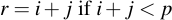

Subtraction is equally easy: just subtract the two values. If the result is less than zero, simply add p, i.e.:

1.2.1 Example
- 13 + 57 = 70 mod 101
- 13 + 9 = 22 mod 23
- 13 - 57 = 57 mod 101
- 13 - 9 = 4 mod 23
1.3 Multiplication
For multiplication of two integers i and j of bitlength b, the result will have a worst-case bitlength of 2b. After each multiplication operation the whole integer has to be taken modulo p. This is already non-trivial: Continuously subtracting p from the result of the multiplication will give you the desired result, but will not be very efficient. Multiplication can however be reduced to a set of additions using this algorithm:
n = i
r = 0
for (bit = 0; bit < bitlength; bit++) {
    if (bitset(j, bit)) {
        r = (r + n) mod p
    }
    n = (n + n) mod p
}
Or (actual, working Python code):
def multiply(i, j):
    n = i
    r = 0
    for bit in range(bitlength):
        if (j & (1 << bit)):
            r = (r + n) % p
        n = (n + n) % p
    return r
Therefore, we need only log(p) operations to iterate over all bits. Mathematically what happens is that the value j is split up into its power-two components, i.e.:

The intermediate value n is initialized to i at the beginning of the program:

And by adding the value repeatedly to itself, it is doubled every time:
Those parts of the overall sum which are needed for the final result (i.e. where the appropriate bit is set within j) are then added into r, the other ones are discarded.
1.3.1 Example
- 13 * 9 = 2 mod 23
- 13 * 57 = 34 mod 101
- 123 * 456 = 4 mod 2003
- 123 * 456 = 33 mod 101
1.4 Division
To implement division in Fp one first can write the division operation a bit differently:
So instead of dividing directly, we replace that operation by multiplication with the inverse element of the dividend. Multiplication is an operation we can already perform, as shown in the previous section. Also, each element has to have an inverse element, as stated by the basic rules of the group Fp. Finding it is a bit tricky, however. We use the extended euclidian algorithm to perform this (you guessed it: working Python code!):
def eea(i, j):
    assert(isinstance(i, int))
    assert(isinstance(j, int))
    (s, t, u, v) = (1, 0, 0, 1)
    while j != 0:
        (q, r) = (i // j, i % j)
        (unew, vnew) = (s, t)
        s = u - (q * s)
        t = v - (q * t)
        (i, j) = (j, r)
        (u, v) = (unew, vnew)
    (d, m, n) = (i, u, v)
    return (d, m, n)
Performing the EEA on any two integers i, j will yield their greatest common divisor d (which we're not particularly interested in) and the Bézout-coefficients m, n. These coefficients have a special meaning:
This means in other words: If we use the EEA on (p, j), d will be 1 since p is prime. The resulting Bézout-coefficient will fulfill the following equation:
Therefore, m is exactly the inverse element of j modulo p. After performing the EEA, we therefore have to only multiply (which we can already do):
1.4.1 Example
- 77 / 13 = 37 mod 101
- EEA(101, 13): d = 1, m = -31, n = 4
- 13-1 = -31 mod 101 = 70 mod 101
- Check: 13 * 70 = 1 mod 101
- 13 / 77 = 71 mod 101
- EEA(101, 77): d = 1, m = 21, n = -16
- 77-1 = 21 mod 101
- Check: 77 * 21 = 1 mod 101
- 123 / 1234 = 1758 mod 2003
- EEA(2003, 1234): d = 1, m = 112, n = -69
- 1234-1 = 112 mod 2003
- Check: 1234 * 112 = 1 mod 2003
1.5 Exponentiation
The last operation which we will want to perform efficiently is modular exponentiation. Luckily, this works in much the same way that we already implemented multiplication.
n = i
r = 1
for (bit = 0; bit < bitlength; bit++) {
    if (bitset(j, bit)) {
        r = (r * n) mod p
    }
    n = (n * n) mod p
}
Or again in real, working Python code:
def exponentiate(i, j):
    n = i
    r = 1
    for bit in range(bitlength):
        if (j & (1 << bit)):
            r = multiply(r, n)
        n = multiply(n, n)
    return r
This is also called the square-and-multiply approach -- but it's nothing really fancy. To understand what's going on, it is necessary to keep in mind the exponentiation rules which are:
Then what we are performing algorithmically is very similar to the trick that we already did with multiplication. Only here the exponent j is split up into it's power-two-components, i.e.:

When multiplying a number with itself, (i.e. the n = n * n operation) does

Therefore, starting with the initialization of n, n0 is initialized to i:

And by continuously multiplying the intermediate variable n with itself, all powers of two are iterated.
Those which are needed for use in the final product (i.e. where the bit is set to one) are then multiplied into r, the other intermediate values are ignored.
1.5.1 Example
- 1357 = 45 mod 101
- 1358 = 80 mod 101
- 1359 = 30 mod 101
- 7799 = 21 mod 101
- 210 = 14 mod 101
- 220 = 95 mod 101
- 230 = 17 mod 101
- 240 = 36 mod 101
- 314159265359271828182846 = 122574892404968648570787373191368149806 mod (2127 - 1)
1.6 Square Root
Finding the square root to a number within Fp is not necessary for doing usual ECC arithmetic, but may be useful notetheless. If you look at the ECC equation, you'll see that a term y2 appears within -- if we ever want to solve for y, we would need modular square rooting. This is much harder than it sounds, actually. Given a number x in Fp, for which we assume that it is a square (also known as "a quadratic residue modulo p"):
we're looking for a y so that
Note that the square root symbol has nothing to do with a square root over R or even C. It is a function which may or may not have a result. Finding the square root, as I mentioned, can be difficult -- but if p is 3 congruent modulo 4, it can be really easy. That is, if:
"Huh?" I hear you say. It sounds bizarre. Let's look at the math. Consider a specific power of x:

Or, in other terms:

Now we apply Fermat's little theorem, which says that
Therefore
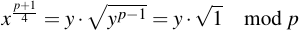
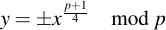
The square root of 1 exists in all Fp, and has the two results 1 and -1 (or in other words, p - 1). Substitution therefore yields
But how can we decide from any given number if it is a quadratic residue over Fp? One way is to simply check by squaring the candidate for y and see if the result is x. Another way is by calculating the so-called Legendre symbol before determining the candidate. The Legrende symbol is given by the formula
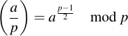
This is not to be confused with division (which would be division by zero). The Legrende symbol has only three possible values: -1, 0 and 1. It is zero when a is 0 mod p (this is the not-so-interesting case). But it is 1 if a is a quadratic residue modulo p and -1 if a is a quadrativ non-residue modulo p. In other words: If there is a square root of any given a, the Legrende symbol will be 0 or 1, otherwise it will be -1.
But what if p is not 3 modulo 4? Well, then one way to solve the problem is by application of the Tonelli–Shanks algorithm, which you can find on Wikipedia and which is also quite straightforward.
2 Elliptic Curve Cryptography
2.1 Introduction
If you're first getting started with ECC, there are two important things that you might want to realize before continuing:
- "Elliptic" is not elliptic in the sense of a "oval circle".
- "Curve" is also quite misleading if we're operating in the field Fp. The drawing that many pages show of a elliptic curve in R is not really what you need to think of when transforming that curve into Fp. Rather than a real "curve" (i.e. a not-straight line), it is more like a cloud of points in the field -- these points are not connected.
Rather than getting confused by the meaning of the words which you might assume, rather try to get confused by the mathematically correct definition of a "Elliptic Curve": it's a smooth, projective algebraic curve of genus one and third degree with a distinct point O (at infinity). Or maybe just ignore the term and continue -- it's not really necessary to get it running and you'll see where this is going anyways. Maybe it will all make sense in the end.
2.2 Elliptic Curve Equation
If we're talking about an elliptic curve in Fp, what we're talking about is a cloud of points which fulfill the "curve equation". This equation is:
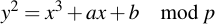
Here, y, x, a and b are all within Fp, i.e. they are integers modulo p. The coefficients a and b are the so-called characteristic coefficients of the curve -- they determine what points will be on the curve.
Note that the curve coefficients have to fulfill one condition:
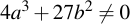
This condition guarantees that the curve will not contain any singularities.
2.3 Point representation
Representing a point on the curve is most intuitively done in the so-called affine projection. Points which are represented in affine coordinates are vectors with an x and y component, just like in an euclidian coordinate system. The only difference is that the x and y values are also integers modulo p. There is one exception: One point at infinity, called O, is present on any curve. To denote points, uppercase letters will be used -- to denote integers, lowercase letters will come into play:

3 Point Operations
To do any meaningful operations on a elliptic curve, one has to be able to do calculations with points of the curve. The two basic operations to perform with on-curve points are:
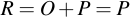
- Point addition: R = P + Q
- Point doubling: R = P + P
Out of these operations, there's one compound operation, scalar point multiplication, which can be implemented by the two above. This will also be described. Note that adding any point to the special point at infinity yields the point, or mathematically speaking:
3.1 Point Addition
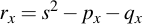
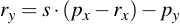
Adding two points is not as easy as simply adding their x- and y-components and taking them modulo p. Instead it is more like connecting the two points via a line and then intersecting that line with the curve (although this operation will not yield the resulting point, but its conjugate). What it exactly relates to is not really important, however. What is important is how you perform the calculation based on what you've already implemented. Note that point addition only works on two points which are not the same:
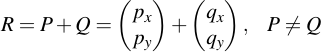
Then, you need to perform the following calculations:

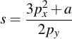
3.2 Point Doubling
Point doubling comes into play if two points shall be added which are identical, i.e.:

These are the calculations needed to get R. Note that a, which is needed for calculating s, is one of the curve parameters:
3.3 Scalar Point Multiplication
When point multiplication and point doubling are implemented, one can derive from those two basic building blocks scalar point multiplication, i.e. multiplying a scalar value (a integer) with a point:

The trick works surprisingly similar to the method we already used to achieve integer multiplication:
N = A
R = O    // Point at infinity
for (bit = 0; bit < bitlength; bit++) {
    if (bitset(k, bit)) {
        R = point_add(R, N)
    }
    N = point_double(N)
}
The inverse of that operation, i.e. finding k for a given A and R, is called the "discrete logarithm". This is an operation which is (without any further tricks like knowing a secret "helper" value) considered computationally infeasible. Therefore it lays the foundation for the ECC cryptosystem: Finding R for given k and A is easy, the opposite direction is hard -- unless you have the "helper" value called "private key".
3.4 Checking if a point is on curve
A good way to check your results for plausibility is to check if the result of a point addition or scalar point multiplication yields in a point which is again on the curve. How can you do this? Well, it is really surprisingly easy -- for a point A to check if it's on the curve, you only need to plug its vector components into the curve equation and see if it all works out:

4 Doing useful ECC operations
4.1 Curve cryptosystem parameters
In order to turn all these mathematical basics into a cryptosystem, some parameters have to be defined that are sufficient to do meaningful operations. There are 6 distinct values for the Fp case and they comprise the so-called "domain parameters":
- p: The prime number which defines the field in which the curve operates, Fp. All point operations are taken modulo p.
- a, b: The two coefficients which define the curve. These are integers.
- G: The generator or base point. A distinct point of the curve which resembles the "start" of the curve. This is either given in point form G or as two separate integers gx and gy
- n: The order of the curve generator point G. This is, in layman's terms, the number of different points on the curve which can be gained by multiplying a scalar with G. For most operations this value is not needed, but for digital signing using ECDSA the operations are congruent modulo n, not p.
- h: The cofactor of the curve. It is the quotient of the number of curve-points, or #E(Fp), divided by n.
4.2 Generating a keypair
Generating a keypair for ECC is trivial. To get the private key, choose a random integer dA, so that

Then getting the accompanying public key QA is equally trivial, you just have to use scalar point multiplication of the private key with the generator point G:
Note that the public and private key are not equally exchangeable (like in RSA, where both are integers): the private key dA is a integer, but the public key QA is a point on the curve.
4.3 Encrypting using ECIES
4.3.1 Encryption
Performing encryption using ECIES is then relatively easy. Let's assume we want to encrypt data with the public key QA that we just generated. Again, first choose a random number r so that

Then, calculate the appropriate point R by multiplying r with the generator point of the curve:

Also multiply the secret random number r with the public key point of the recipient of the message:

Now, R is publicly transmitted with the message and from the point S a symmetric key is derived with which the message is encrypted. A HMAC will also be appended, but we'll skip that part here and just show the basic functionality.
4.3.2 Decryption
Now assume that you receive a message, which is encrypted with a symmetric key. Together with that message you receive a value of R in plain text. How can you -- with the aid of your private key, of course -- recover the symmetric key? Well, that's also easy:

By just multiplying your private key with the publicly transmitted point R, you will receive the shared secret point S, from which you can then derive the symmetric key (with the same mechanism that the sender did generate it, of course).
To see why this works so beautifully, you just have to take a look at the equations and substitute:

4.4 Signing using ECDSA
4.4.1 Signing
Generating and verifying signatures via ECDSA is a little bit more complicated that encrypting data, but it's not impossible to understand. Again, let's assume that we have a keypair QA, dA and want to sign a message with our private key. First, we calculate a hash value of the message that we're about to sign. For this for example SHA-1 can be used:
Then, as with ECIES, a random number has to be generated (here it's called k, not r). This random number must under all circumstances be different for each generated signature, or the private key pair can be regenerated with some tricks (you'll see later on why):

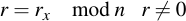
This number k is then multiplied with the generator point G of the curve and the x coordinate is taken modulo n:
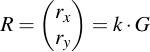
Note that this is the exact same process as key generation, with a new private key k. In fact, the values (k, R) are also in some documents referred to as "ephemeral" or temporary keypairs.
If r is 0, a new random number has to be chosen. If a r not equal to 0 has been found, s can be calculated:
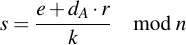
If s is 0, a new random number has to be chosen. If it is not equal to zero, the resulting pair of two integers (r, s) is then the final signature.
4.4.2 Signature Verification
Now for the opposite direction: You received a message m, a signature (r, s) and have the public key QA of the supposed sender. Now is the message legit? Let's check it by first verifying that the values or (r, s) are plausible. If they're not, the signature is invalid:

Now that these values are okay, generate the hash value of the message:
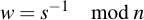
Then invert s (modulo n):
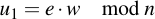
And calculate two integers u1 and u2:
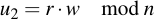
Then calculate the point P using the results of these computations:
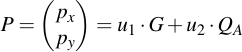
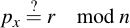
And take px modulo n. The signature is valid if px is equal to the received r (modulo n):
4.4.3 Why ECDSA works
Now since these calculations are not immediately obvious, I will try to explain why they work. Let's start at the signature verification equation:
Then, substitute u1 and u2:

Substitute QA for the definition of the public key:

Now factor G and w:

Remember the definition of w:
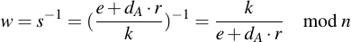
And substitute into the equation of P -- rhe term e + dAr nicely cancels out:
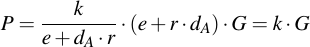
During signature creation, kG was exatly the definition of R. Only the X-component of that point is transmitted, which is obiously equal (since the points R and P are equal for a correct signature).
4.5 Messing with ECDSA signatures
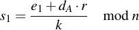
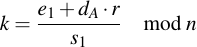
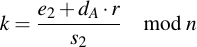
This is one of the most fun parts and actually the reason why I wanted to understand ECC -- to be able to understand how to mess with them. As we've seen in the chapter about signature generation, for each distinct signature a different nonce k value has to be used. This is important because of the following reason: Let's say we have two messages m1 and m2 which are both signed with an identical nonce k. This means the value of r will be the same for both signatures, they will only have different values of s, s1 and s2. These values are:
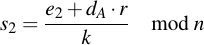
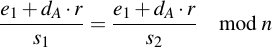
Note that there are only two unknowns in these equation: dA and k. Since we have two equations and two unknowns, we can solve for dA and k. First rearrange the above equations:
Then set them equal and solve:
Multiply with s1 s2:

Expand left and right side:

Subtract s1 e2 and s2 dA r:

Factorize the right side:

And divide everything by r (s1 - s2):
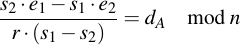
After we have calculated the private key, for fun and profit we can also calculate the "random" nonce which was used:
This works equally well with e2 or s2, of course.
4.5.1 Excursion: Some of Sony's unwise choices
In Console Hacking 2010 - PS3 Epic Fail, fail0verflow describe multiple hacks against Sony's PlayStation 3 console. One of them was against signed binaries that Sony uses to be able to run trusted code only. In other words: You cannot just run any program on a PlayStation 3, but you have to give it to someone with the signing key, who will review the code. Then, after it's been approved, they sign your binary. The Sony bootloader then first checks the signature of the binary (to see if it's approved to run) and only runs the binary if the signature checks out.
Now the problem is that Sony did not realize the importance of having a distinct nonce for every single signature they pass out. Instead, they opted for the "one nonce suits all" option. This itself is stupid, but admittedly forgivable (since the disastrous implications are not immediately obvious in my opinion). What is not forgivable, however, is what followed: Being caught with their pants down, they decided that it was the hacker's fault. Consequently, they decided to sue George Hotz and fail0verflow and prosecute anyone who posted the (now public) private key of theirs.
That's a prime example of douchey corporate behavior. If you mess up, at least don't be such a cry-baby about it. Don't blame others for your own screw-ups.
5 Advanced Topics
5.1 Point Compression
To do actual work with points, they have to be stored in their complete (explicit) form. To just uniquely identify a point which is on the curve, giving its canonical coordinates is not necessary. Since we know that a point is on-curve, it is in sufficient to only store the x-coordinate and the least significant bit of the y-coordinate. This can be done in the manner described in the SECG document, section 2.3.3 and following. First, consider a point P and its compressed pendant P roof:
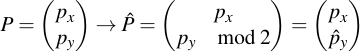
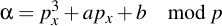
As you can see, P is very easily compressed by leaving px as it is and just taking py modulo 2, i.e. reducing it to its least significant bit. Regenerating the original point is a little bit more challenging. First calculate a helper value α:
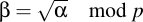
Then perform the discrete square root to yield two (or no) values of β:
If this fails, then an invalid x coordinate was given and the point compression is invalid. But if the point was correctly compressed, this square rooting yields two values:
![latex:\beta = [ \beta_1, \beta_2 ]](tex/75997755200ebb19d2a0a3ceb87d81fa.png)
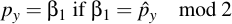
Now you take β1 modulo 2 and see if it is equal to the compress py. If so, then β1 is the wanted py. Otherwise, β2 is the wanted py:
6 Examples
6.1 Testing your integer arithmetic using Genius
If you would like to verify if your implementation of modular integer arithmetic is correct, it is tremendously useful to compare your results against other implementations. For this I can highly recommend the GPLed math-tool Genius. With Genius you can easily recap all calculations and see if your results turn out. It supports the four basic modular operations, exponentiation and square rooting. Plus: it is really easy to use! Here's an example:
joequad joe [~]: genius --maxdigits=0
Genius 1.0.11
Copyright (C) 1997-2010 Jiří (George) Lebl, Ph.D.
This is free software with ABSOLUTELY NO WARRANTY.
For license details type `warranty'.
For help type 'manual' or 'help'.

genius> 123^456 mod 2003
= 635
genius> 77^-1 mod 101
= 21
genius> 12^-1 mod 101
= 59
genius> p = (2^127) - 1
= 170141183460469231731687303715884105727
genius> IsPrime(p)
= true
genius> 123456^123456 mod p
= 29297808435319758216633793520210693282
genius>
6.2 Using Sage to play with elliptic curves
Sage, for me as a Python programmer, is a dream come true: It's a very capable and powerful CAS which uses Python: Therefore, all calculations are done using Python syntax and you can use all the power of Python do achieve what you want. It absolutely blew my socks off when I first used it. When you register at their website, you can even try it out online without having to install it locally. Wow!
Anyways, let's start some modular arithmetic. In Sage, the field is always defined explicitly (I've added empty lines and comments for better readability):
----------------------------------------------------------------------
| Sage Version 4.7.1, Release Date: 2011-08-11                       |
| Type notebook() for the GUI, and license() for information.        |
----------------------------------------------------------------------
sage: F = FiniteField(17)                  # Generate a finite field
sage: print(F)
Finite Field of size 17

sage: F(3)                                 # Generate an integer over the field
3
sage: type(F(3))                           # Show its type
<type 'sage.rings.finite_rings.integer_mod.IntegerMod_int'>

sage: F(3) * 123                           # Do modular multiplication
12

sage: F(3) ^ -1                            # Do modular inversion
6
sage: F(3) * 6                             # Check the result for correctness
1

sage: F(8).sqrt()                          # Square root an invertible integer
5
sage: F(5) * 5                             # Check the result
8

sage: F(3).sqrt()                          # Square root a non-invertible integer
sqrt3
sage: (F(3).sqrt()) ^ 2                    # Check the result
3
Note that you can even calculate with values like the square root of 3 over F17 even though it does not have an explicit representation in F17 -- this is really cool!
Now let's place an elliptic curve in a prime field. Sage does not only understand elliptic curves of the form
But is capable of much, much more. Curves in Sage have the form of (see the excellent Sage docs for more info on that):

Now obviously, if you set
You will still receive a curve in the so-called short Weierstraß form (which is what we will use). Let's first start with a tiny curve (we will also use that curve later on):
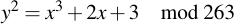
sage: F = FiniteField(263)                  # Generate a finite field
sage: C = EllipticCurve(F, [ 2, 3 ])        # Set a, b
sage: print(C)
Elliptic Curve defined by y^2 = x^3 + 2*x + 3 over Finite Field of size 263

sage: print(C.cardinality())                # Count number of points on curve
270

sage: print(C.points()[:4])                 # Show the first four points
[(0 : 1 : 0), (0 : 23 : 1), (0 : 240 : 1), (1 : 100 : 1)]
Note that sage represents points with three coordinates. The third coordinate tells us whether the point is at infinity (if it's 0) or not (then it is 1). Let's choose a generator point, take (200, 39):
sage: G = C.point((200, 39))
sage: G
(200 : 39 : 1)
sage: G.order()
270
We know the order is 270, that means that when multiplying scalars with G there is a total of 270 unique points that will be the result (i.e. 269 plus one at infinity). Since this is equal to the number of points on the curve, we know that by choosing this generator, every single point will be used. This is by far not always the case. Let's choose a second generator point H with a low order. Looking for low-order points is easy using Python magic. Let's look for all points with an order smaller than 10:
sage: [ p for p in C.points() if (p.order() < 10) ]
[(0 : 1 : 0), (60 : 48 : 1), (60 : 215 : 1), (61 : 20 : 1), (61 : 243 : 1),
(102 : 90 : 1), (102 : 173 : 1), (126 : 76 : 1), (126 : 187 : 1),
(128 : 81 : 1), (128 : 182 : 1), (144 : 35 : 1), (144 : 228 : 1),
(175 : 83 : 1), (175 : 180 : 1), (262 : 0 : 1)]
Now let's also get their order as tuples (did I mention that I love Python?):
sage: [ (p.order(), p) for p in C.points() if (p.order() < 10) ]
[(1, (0 : 1 : 0)), (9, (60 : 48 : 1)), (9, (60 : 215 : 1)), (5, (61 : 20 : 1)),
(5, (61 : 243 : 1)), (9, (102 : 90 : 1)), (9, (102 : 173 : 1)),
(6, (126 : 76 : 1)), (6, (126 : 187 : 1)), (9, (128 : 81 : 1)),
(9, (128 : 182 : 1)), (3, (144 : 35 : 1)), (3, (144 : 228 : 1)),
(5, (175 : 83 : 1)), (5, (175 : 180 : 1)), (2, (262 : 0 : 1))]
Let's sort them by order ascending:
sage: sorted([ (p.order(), p) for p in C.points() if (p.order() < 10) ])
[(1, (0 : 1 : 0)), (2, (262 : 0 : 1)), (3, (144 : 35 : 1)),
(3, (144 : 228 : 1)), (5, (61 : 20 : 1)), (5, (61 : 243 : 1)),
(5, (175 : 83 : 1)), (5, (175 : 180 : 1)), (6, (126 : 76 : 1)),
(6, (126 : 187 : 1)), (9, (60 : 48 : 1)), (9, (60 : 215 : 1)),
(9, (102 : 90 : 1)), (9, (102 : 173 : 1)), (9, (128 : 81 : 1)),
(9, (128 : 182 : 1))]
Let's choose (126, 76) as our weak generator point H. Then show all the points that are iterated when multiplying scalars with H:
sage: H = C.point((126, 76))
sage: H.order()
6
sage: pts = [ H * x for x in range(H.order()) ]
sage: pts
[(0 : 1 : 0), (126 : 76 : 1), (144 : 35 : 1), (262 : 0 : 1), (144 : 228 : 1), (126 : 187 : 1)]
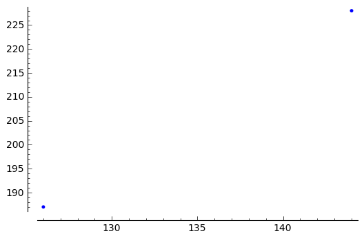
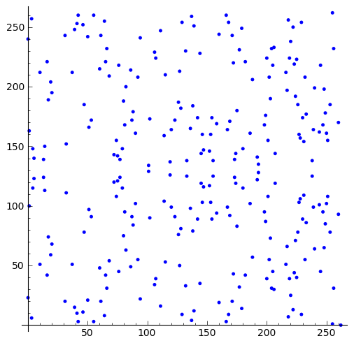
As you might have guessed, Sage can also plot these points. Let's first plot a single point:
sage: pts[4]
(144 : 228 : 1)
sage: plot(pts[4])
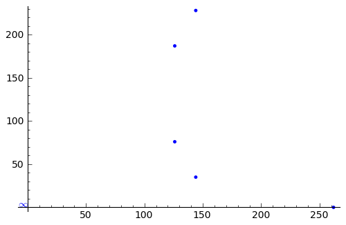
Plotting multiple things is done by adding plots in Sage. Consequently we will be able to use the sum-function to plot all points!
sage: plot(pts[4]) + plot(pts[5])
sage: sum([ plot(p) for p in pts ])
Let's color those subgroup points created by H in orange:
sage: plot1 = sum([ plot(p, hue = 0.1) for p in pts ])
sage: plot1
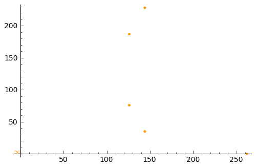
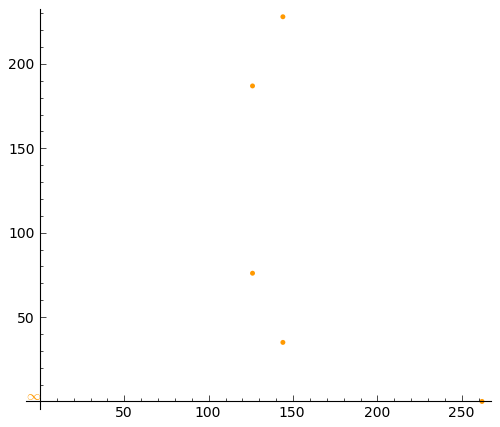
Since X and Y should have a 1:1 ratio, let's do this:
sage: plot(plot1, aspect_ratio = 1)
Let's also plot all points on the curve:
sage: plot(C, aspect_ratio = 1)
Let's plot all points (in blue) together with the points of the subgroup created by the weak generator point H:
sage: plot((plot(C) + plot1), aspect_ratio = 1)
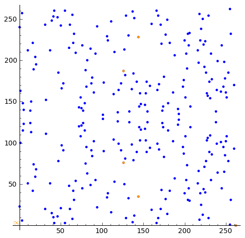
Now if that isn't cool I don't know what is :-)
6.3 Extracting curve parameters from openssl
If you want to play with real curves, a good source is openssl. To first check what curves your openssl variant supports, you can easily list then:
joequad joe [~]: openssl ecparam -list_curves
  secp112r1 : SECG/WTLS curve over a 112 bit prime field
  secp112r2 : SECG curve over a 112 bit prime field
  secp128r1 : SECG curve over a 128 bit prime field
  secp128r2 : SECG curve over a 128 bit prime field
  secp160k1 : SECG curve over a 160 bit prime field
[...]
All curves which are specified over a "prime field" are exactly what we did all the time, a curve over Fp. Curves over binary fields are not discussed here. So choose one of your liking (I'll take secp112r1) and display its parameters:
joequad joe [~]: openssl ecparam -param_enc explicit -conv_form uncompressed -text -noout -no_seed -name secp112r1
Field Type: prime-field
Prime:
    00:db:7c:2a:bf:62:e3:5e:66:80:76:be:ad:20:8b
A:
    00:db:7c:2a:bf:62:e3:5e:66:80:76:be:ad:20:88
B:
    65:9e:f8:ba:04:39:16:ee:de:89:11:70:2b:22
Generator (uncompressed):
    04:09:48:72:39:99:5a:5e:e7:6b:55:f9:c2:f0:98:
    a8:9c:e5:af:87:24:c0:a2:3e:0e:0f:f7:75:00
Order:
    00:db:7c:2a:bf:62:e3:5e:76:28:df:ac:65:61:c5
Cofactor:  1 (0x1)
By removing all the colons, you already have the numbers you want in hexadecimal representation. Note that for the generator point G in uncompressed form you have to discard the first byte (0x04 indicates that the two points are encoded directly, without compression -- see section 2.3.3 of the SECG document for details), then comes the x- and y-component. So for this example, the values are:


6.4 Playing with openssl ECDSA signatures
OpenSSL by default does not do the same mistake that Sony did with their PS3 signatures. However, it can by changing one line easily be modified to perform the same result. We will demonstrate this in order to show the attack. First we have to Sonyfy OpenSSL. For this, the following patch can be used:
diff -r -c3 openssl-1.0.0d-orig//crypto/ecdsa/ecs_ossl.c openssl-1.0.0d/crypto/ecdsa/ecs_ossl.c
*** openssl-1.0.0d-orig//crypto/ecdsa/ecs_ossl.c    2009-12-01 18:32:33.000000000 +0100
--- openssl-1.0.0d/crypto/ecdsa/ecs_ossl.c    2011-09-29 20:14:20.000000000 +0200
***************
*** 134,148 ****

      do
      {
!         /* get random k */
!         do
!             if (!BN_rand_range(k, order))
!             {
!                 ECDSAerr(ECDSA_F_ECDSA_SIGN_SETUP,
!                  ECDSA_R_RANDOM_NUMBER_GENERATION_FAILED);
!                 goto err;
!             }
!         while (BN_is_zero(k));

          /* compute r the x-coordinate of generator * k */
          if (!EC_POINT_mul(group, tmp_point, k, NULL, NULL, ctx))
--- 134,141 ----

      do
      {
!         /* get not so random k, hahaha */
!         BN_set_word(k, 0x536f6e79);        /* Sonyfy ECDSA security! */

          /* compute r the x-coordinate of generator * k */
          if (!EC_POINT_mul(group, tmp_point, k, NULL, NULL, ctx))
Therefore, after a random number has successfully been chosen, we simply override it with the constant value 0x536f6e79. Then, let's generate a keypair first:
joequad joe [~/sonyecc]: openssl ecparam -name secp192k1 -genkey -out sony.key
After the key has been created, let's create a X.509 certificate from that key:
joequad joe [~/sonyecc]: openssl req -new -x509 -nodes -days 365 -key sony.key -out sony.crt
[...]
Then, let's sign some data using S/MIME. Be sure to used your Sonyfied version of OpenSSL:
joequad joe [~/sonyecc]: echo -n foo | ./openssl smime -sign -signer sony.crt -inkey sony.key -noattr -out foo.sig
joequad joe [~/sonyecc]: echo -n bar | ./openssl smime -sign -signer sony.crt -inkey sony.key -noattr -out bar.sig
Convert the S/MIME blobs into PKCS7 (apparently in version 1.0.0 this does not work in the same step):
joequad joe [~/sonyecc]: openssl smime -pk7out -in foo.sig -out foo.pk7
joequad joe [~/sonyecc]: openssl smime -pk7out -in bar.sig -out bar.pk7
Then examine the signature blob of the foo signature first by using the ASN1 decoder of OpenSSL:
joequad joe [~/sonyecc]: openssl asn1parse -in foo.pk7
[...]
  810:d=5  hl=2 l=   9 cons: SEQUENCE
  812:d=6  hl=2 l=   5 prim: OBJECT            :sha1
  819:d=6  hl=2 l=   0 prim: NULL
  821:d=5  hl=2 l=   9 cons: SEQUENCE
  823:d=6  hl=2 l=   7 prim: OBJECT            :ecdsa-with-SHA1
  832:d=5  hl=2 l=  56 prim: OCTET STRING      [HEX DUMP]:3036021900B44654432124B9EE0CAE954630AE09B5FB0D81A350005F25021900B0035643E4C581DC089278F4E661F0FB7F98F14E8FA81785
You can see that the signature is the last octet string in the tuple, it encodes r and s. In my example this octet string starts at offset 832, but YMMV. To further decode that octet string:
joequad joe [~/sonyecc]: openssl asn1parse -in foo.pk7 -strparse 832
    0:d=0  hl=2 l=  53 cons: SEQUENCE
    2:d=1  hl=2 l=  25 prim: INTEGER           :B44654432124B9EE0CAE954630AE09B5FB0D81A350005F25
   29:d=1  hl=2 l=  25 prim: INTEGER           :B0035643E4C581DC089278F4E661F0FB7F98F14E8FA81785
Then, do the same for the bar.pk7:
joequad joe [~/sonyecc]: openssl asn1parse -in bar.pk7 -strparse 832
    0:d=0  hl=2 l=  54 cons: SEQUENCE
    2:d=1  hl=2 l=  25 prim: INTEGER           :B44654432124B9EE0CAE954630AE09B5FB0D81A350005F25
   29:d=1  hl=2 l=  24 prim: INTEGER           :3EE09F92DD92BBCAE1BFFB9708115E66850A2AD33F394DD8
You can already see that the values for r are identical for both signatures -- so this is going to be fun! First, let's again see what key we have created before. For this, you need to decode the ASN1 part of the keyfile which says "EC PRIVATE KEY" (not the "EC PARAMETERS"):
joequad joe [~/sonyecc]: cat sony.key | tail -n +4 | openssl asn1parse
    0:d=0  hl=2 l=  92 cons: SEQUENCE
    2:d=1  hl=2 l=   1 prim: INTEGER           :01
    5:d=1  hl=2 l=  24 prim: OCTET STRING      [HEX DUMP]:EC7C14196B64ABEA2E70D52002EF8E01748252B060D8E980
   31:d=1  hl=2 l=   7 cons: cont [ 0 ]
   33:d=2  hl=2 l=   5 prim: OBJECT            :secp192k1
   40:d=1  hl=2 l=  52 cons: cont [ 1 ]
   42:d=2  hl=2 l=  50 prim: BIT STRING
Then, let's recap what signature values the messages have. They are included in the PKCS7 (you can read them out via the decoded ASN1), or you can just simply calculate them using sha1sum:
joequad joe [~/sonyecc]: echo -n foo | sha1sum
0beec7b5ea3f0fdbc95d0dd47f3c5bc275da8a33  -
joequad joe [~/sonyecc]: echo -n bar | sha1sum
62cdb7020ff920e5aa642c3d4066950dd1f01f4d  -
And let's also dump the domain parameters of the secp192k1 curve:
a = 0
b = 3
p = 0xfffffffffffffffffffffffffffffffffffffffeffffee37
n = 0xfffffffffffffffffffffffe26f2fc170f69466a74defd8d
h = 1
gx = db4ff10ec057e9ae26b07d0280b7f4341da5d1b1eae06c7d
gy = 9b2f2f6d9c5628a7844163d015be86344082aa88d95e2f9d
Then, using the Python scripts I wrote (downloadable below in the package called joeecc), create that curve in Python:
secp192k1 = curves["secp192k1"]
recvr = secp192k1.exploitidenticalnoncesig(
    0xB44654432124B9EE0CAE954630AE09B5FB0D81A350005F25,
    0x0ADA8B0EB836F72A00072936ACABECD00EC6BF5114B35FFA,
    "foo",
    0x99B7D45DB1043118D934ABD6F54E565223A13F40392393DA,
    "bar"
)
print("Recovered nonce      : 0x%x" % (recvr["nonce"].getintvalue()))
print("Recovered private key: 0x%x" % (recvr["privatekey"].getintvalue()))
...just let it run and watch the fun...
Recovered nonce      : 0x536f6e79
Recovered private key: 0xec7c14196b64abea2e70d52002ef8e01748252b060d8e980
Yippey!
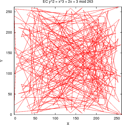
6.5 Visualizing a small curve
In order to better understand the underlying nature of a curve, consider this very tiny curve:
With the generator base point:

Just showing the points on the curve looks kind of tidy:
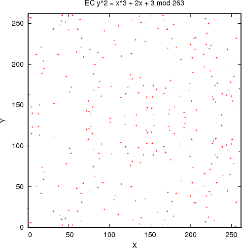
But when they're connected with lines in the order they appear on the curve (as generated by the generator base point G), this does not look so tidy anymore -- it is quite chaotic:
7 FAQ
7.1 Cool! Now that I know how to use ECC, should I write my own crypto library?
Please don't. This tutorial is meant to merely help people understand how the underlying crypto works. It is not meant to be used productively at all! Please understand that the people who do write crypto libraries for a living have an incredible amount of knowledge about all kinds of topics that are relevant to ensure security in a real-world scenario. If you don't know your stuff, do not expect to write code that is secure (although it might give the false impression of being secure).
7.2 Can I at least define my own curve then?
Please don't. As with the answer to the previous question, people who define curves and choose generator points really know what they're doing. They have years of experience (and probably one or two Ph.D.s in mathematics more than you). Do not expect to produce high-quality curves with just the aid of some web tutorial.
7.3 But I don't trust NIST/SECG. What alternatives do I have?
Have a look at the Brainpool curves if you're looking for Short Weierstrass curves. They are provably randomly chosen, so the possibility that someone has hidden a backdoor in them is extremely unlikely.
If you're up for newer stuff, check out Daniel J. Bernstein's Curve25519, which is a Twisted Edwards curve and uses a signature scheme different from the ECDSA shown here. Twisted Edwards curves are getting traction quite quickly. Another interesting curve is Ed448-Goldilocks, if you're looking for a larger base field.
7.4 Your implementation isn't side channel resistant, hurr durr!
Great observation, and true as well, yes. The computations here and the implementation of joeecc don't care about side channel resistance because they're not meant to show a productive implementation. They're merely intended to explore the involved math and demonstrate the concept. Apart from that, please refer to question 7.1.
8 Downloads
| Filename | Last Changed | Description |
|---|---|---|
|
joeecc on GitHub Release v0.05 from 2015-08-12 |
2015-08-11 |
|
| simplemodarith.py | 2011-09-29 |
|
| tcdata_modarith.txt.gz | 2011-09-29 |
|
| tcdata_curve.txt.gz | 2011-09-29 |
|
| openssl_sonyfy.patch | 2011-09-29 |
|
| ecdsa-identical-nonce-hack.tar.gz | 2011-09-29 |
|
| pointcloud.tar.gz | 2011-09-29 |
|
9 Literature
| Document | Author | Description |
|---|---|---|
| Elliptic Curve Cryptography - An Implementation Guide | Anoop MS |
|
| SEC 1: Elliptic Curve Cryptography | SECG |
|
| ECC Tutorial | Certicom |
|
| Console Hacking 2010 - PS3 Epic Fail | fail0verflow |
|
| RFC3279: Algorithms and Identifiers for the Internet X.509 Public Key Infrastructure Certificate and Certificate Revocation List (CRL) Profile | W. Polk, R. Housley, L. Bassham |
|